

The paper
Justin Grimmer, Solomon Messing, and Sean J. Westwood (2017). Estimating Heterogeneous Treatment Effects and the Effects of Heterogeneous Treatments with Ensemble Methods. Political Analysis 25(4), 413–434.
doi:10.1017/pan.2017.15 (opens in a new tab) · Replication data: doi:10.7910/DVN/BQMLQW (opens in a new tab)
Main text
p. 414, Introduction
Published
observational studies (Samii, Paler, and Daly 2017).
Correction
observational studies (Samii, Paler, and Daly 2016).
Basis Political Analysis 24(4) is the 2016 volume; see the correction to the references, pp. 433–434.
p. 419, Equation 8 and the sentence after it
Published
Y_i = \sum_{i=1}^{M} w_m \widehat{Y}_{im} + \epsilon_i(8) [...] that the weights sum to 1 (\sum_{i=1}^{M} w_m = 1)Correction
Y_i = \sum_{m=1}^{M} w_m \widehat{Y}_{im} + \epsilon_i(8) [...] that the weights sum to 1 (\sum_{m=1}^{M} w_m = 1)Basis The sums run over the M methods, indexed by m.
p. 421, Section 4
Published
We assess the performance of the ensemble across four distinct data generating processes, averaging the performance of the ensemble over 5 instances of the data generating process. [...] In two simulations, Monte Carlo 1 and Monte Carlo 2 are sparse data generating processes—with many of the simulated treatments specified to have an undetectable systematic effect and only a few specified to have heterogeneous effects. Monte Carlo 3 and Monte Carlo 4, specify data generating processes that are more dense—with more treatments having systematic (and large) effects and heterogeneity across covariates.
Correction
We assess the performance of the ensemble across three distinct data generating processes, averaging the performance of the ensemble over 5 instances of the data generating process. [...] Monte Carlo 1 is a sparse data generating process—with many of the simulated treatments specified to have an undetectable systematic effect and only a few specified to have heterogeneous effects. Monte Carlo 2, Monte Carlo 3 and Monte Carlo 4 specify data generating processes that are more dense—with more treatments having systematic (and large) effects and heterogeneity across covariates. Monte Carlo 2 and Monte Carlo 4 use the same dense design with continuous covariates.
Basis The archived Monte Carlo 2 runs (test_ucs_1-5.RData) reproduce the Monte Carlo 2 column of Table 2 and appendix Table 2, and their data have the dense design. For treatment arms 6–46, whose coefficients the stated sparse design draws from Uniform(−0.07, 0.07), the standard deviation of the arm outcome means is 0.27–0.30 in the five Monte Carlo 2 data sets, 0.26–0.27 in Monte Carlo 4 and 0.04–0.06 in Monte Carlo 1; in 100 data sets simulated from the sparse Monte Carlo 2 design it never exceeds 0.06.
pp. 421–422, Section 4
Published
In the Monte Carlo simulations—and in our applications, below—we form an ensemble with nine methods: (1) LASSO (Hastie, Tibshirani and Friedman 2001); (2) Elastic Net, with the mixing parameter set to 0.5 (Hastie, Tibshirani and Friedman 2001); (3) Elastic Net, with the mixing parameter set to 0.25 (Hastie, Tibshirani and Friedman 2001); [...]
Correction
In the Monte Carlo simulations we form an ensemble with nine methods, and in our applications, below, with seven of them (all but BART and Random Forest): (1) LASSO (Hastie, Tibshirani and Friedman 2001); (2) Elastic Net, with the mixing parameter set to 0.5 (Hastie, Tibshirani and Friedman 2001); (3) ridge regression, the elastic net with the mixing parameter set to 0 (Hastie, Tibshirani and Friedman 2001); [...]
Basis Table 4 and the archived application weights (HetExperimentPreds.RData, BlamePreds.RData) cover seven methods. The archived super-learner code (SLF_round2.R), which RepCode-1.R sources for both applications, fits the third method with
cv.glmnet(..., alpha = 0), which is ridge regression, and stores it as e_net_0.25, the label in the archived weights of all 20 simulation runs and both applications. The same relabeling applies to Tables 2 and 4, p. 423 and the online appendix.p. 422, Table 2
Published
This table presents the mean square error for each method averaged over 5 simulations of each data generating process, divided by the mean square error of the ensemble method average over 5 simulations of each data generating process.
Table 2, “Find It” row: MC 2 17.74, MC 4 25.47, Average 14.66; row label “Elastic Net (α = 0.25)”; and the sentence of the table note quoted above.
Correction
Corrected Table 2, below. The note reads: “This table presents the root mean square error for each method averaged over 5 simulations of each data generating process, divided by the root mean square error of the ensemble method averaged over 5 simulations of each data generating process.”
Corrected Table 2: root mean square error of each method relative to root mean square error of the ensemble. — withdrawn: Find It's Monte Carlo 2 and 4 predictions were not bounded to [0, 1] and applied coefficients estimated on standardized covariates to unstandardized covariates. † includes those Find It predictions with weight 1/9. The Monte Carlo 2 data were generated with the dense design (see the correction to p. 421). Method MC 1 MC 2 MC 3 MC 4 Average LASSO 0.99 1.08 1.34 1.25 1.18 Elastic Net (α = 0.5) 1.03 1.08 1.22 1.14 1.12 Ridge (α = 0) 1.58 1.26 0.95 1.26 1.23 Find It 1.09 — 1.75 — — Bayesian GLM 1.87 1.02 1.10 0.99 1.12 BART 1.08 3.16 1.36 3.65 2.68 Random Forest 4.99 2.05 2.96 2.25 2.64 KRLS 1.53 2.76 1.11 3.31 2.42 SVM-SMO 2.61 2.10 1.77 2.22 2.12 Naive Average 1.38 1.86 † 1.06 2.52 † 1.83 † Basis In the archived prediction code (SLF_round2.R, predict.weight), Find It's coefficients, estimated on standardized covariates, multiply the unstandardized evaluation grid, and the predictions are not bounded to [0, 1], a bound the FindIt package (version 0.3) applies itself. An effect is a difference between two probabilities, so a bounded estimate cannot miss by more than 2, yet the archived Find It RMSEs in Monte Carlo 2 and 4 are 2.47 to 4.00. The archive stores neither the simulated true effects nor the fitted models, so these entries cannot be recomputed and are withdrawn; the same predictions enter the naive average with weight 1/9 (†) and the weighted ensemble with weights of 0.003 to 0.025. Every other method's average ratio is 1.12 or higher.
pp. 422–423, Section 4
Published
Consider the first two columns in Table 2, showing the results for the sparse data generation processes. Here, we see that methods that assume sparsity perform better—methods such as LASSO. [...] The third and fourth columns show that methods that assume a dense set of effects and interactions perform better—such as Elastic Net with α = 0.25, KRLS, and Bayesian GLM.
Correction
Consider the first column in Table 2, showing the results for the sparse data generation process. Here, we see that methods that assume sparsity perform better—methods such as LASSO. [...] The third and fourth columns show that methods that assume a dense set of effects and interactions perform better—such as ridge regression, KRLS, and Bayesian GLM. The second column uses the dense design of the fourth.
Basis Only Monte Carlo 1 uses the sparse design, and the method labeled Elastic Net (α = 0.25) is ridge regression; see the corrections to p. 421.
p. 425, Section 5
Published
gun ranges decrease approval for representatives (13.1 percentage point decrease, 95 percent confidence interval [−0.25, −0.01])
Correction
gun ranges decrease approval for representatives (13.1 percentage point decrease, 95 percent confidence interval [−0.24, −0.02])
Basis Computed as in RepCode-1.R (make.eff), the estimator behind Figure 2: OLS of binary approval on the expenditure-type indicators for the 1,074 respondents, with the interval at ±1.96 standard errors.
p. 427, Table 4
Published
Elastic Net (α = 0.25) 0.00 0.00
Correction
Ridge (α = 0) 0.00 0.00
Basis See the correction to pp. 421–422.
p. 428, Figure 4
Published
Figure 4, both panels: within each project type, the rows labeled “Liberal”, “Moderate” and “Conservative”.
Correction
Corrected Figure 4. In both published panels the rows labeled Moderate show the estimates for conservatives, and the rows labeled Conservative show the estimates for moderates. For the gun range at $20 million, for example, the point printed for moderates (−0.110) is the conservative estimate; the moderate estimate is −0.197.
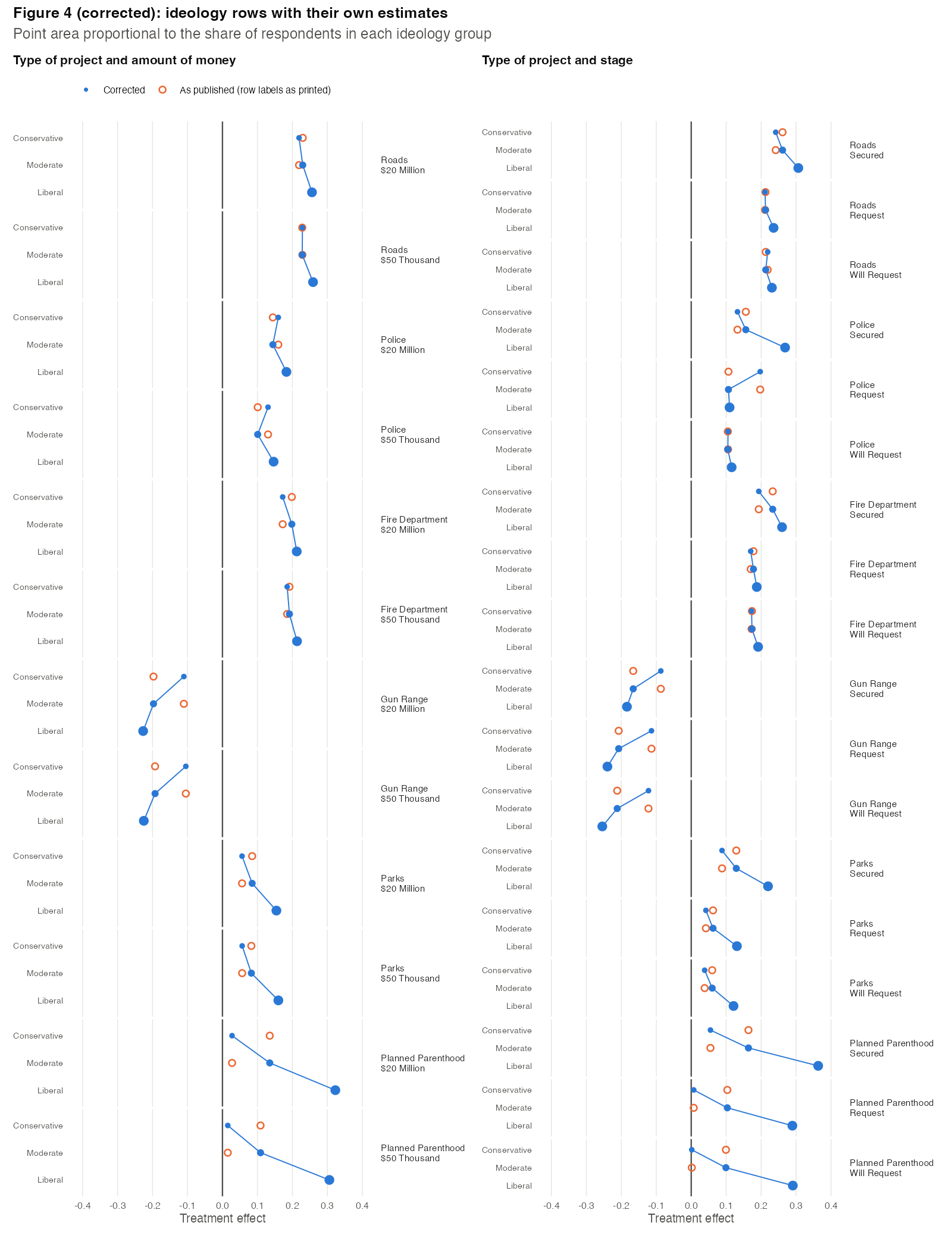
Basis RepCode-1.R codes ideology as 1 = liberal, 2 = conservative and 3 = moderate (ideo_vec2) but passes the row labels and point sizes in the order liberal, moderate, conservative. Hollow points show the published positions. The text's conclusions from Figure 4 do not depend on the ideology labels.
p. 428
Published
claiming credit for a gun range causes only a 5 percentage point decline among conservative Republicans.
Correction
claiming credit for a gun range causes only a 2.6 percentage point decline among conservative Republicans.
Basis Figure 3 plots −0.026 for conservative Republicans (archived ensemble predictions, HetExperimentPreds.RData).
p. 430, Section 5.1
Published
Grimmer, Westwood, and Messing (2014) administered the experiment to 1,166 participants, using a census matched US sample from a Survey Sampling International (SSI) panel.
Correction
Grimmer, Westwood, and Messing (2014) administered the three conditions in Table 5 to 992 participants, using a census matched US sample from a Survey Sampling International (SSI) panel. The ensemble analysis uses the 947 participants with complete covariates and a matched representative ideal point.
Basis The archived data (Public_v_Private_and_Taunting_2.csv) have 2,286 respondents, 992 of them in the three conditions analyzed here; the overall effects reported in this paragraph (8.2 and 7.7 points) reproduce on these 992.
p. 431, Table 6
Published
Table 6. “Democrat Representatives, Most Positive Response”, rows 1 and 2: “Age” 36–49. “Republican Representatives, Most Negative Response”, row 1: “Income” <$50k. “Republican Representatives, Most Positive Response”, row 1: “Party” Republican.
Correction
Corrected Table 6. Rows 1 and 2 of the Democrat most-positive panel have Age 37–49; row 1 of the Republican most-negative panel has Income $50k–$80k; row 1 of the Republican most-positive panel has Party Strong Rep.
Corrected Table 6: characteristics of constituents with the most negative and positive response to budget criticism, from the archived ensemble predictions. Effects to three decimals. Group Effect Education Income Age Gender Race Ideology Party Democrat Representatives, Most Negative Response −0.369 High School $50k–$80k 50–63 Female White Cons. Dem. Democrat Representatives, Most Negative Response −0.361 High School $50k–$80k 64+ Female White Cons. Dem. Democrat Representatives, Most Negative Response −0.357 Grad. Degree $50k–$80k 50–63 Female White Cons. Dem. Democrat Representatives, Most Positive Response 0.280 College <$50k 37–49 Male White Strong Lib. Strong Dem. Democrat Representatives, Most Positive Response 0.271 College <$50k 37–49 Female White Strong Lib. Strong Dem. Democrat Representatives, Most Positive Response 0.267 College <$50k <37 Male White Strong Lib. Independent Republican Representatives, Most Negative Response −0.319 College $50k–$80k 50–63 Male Non-White Strong Cons. Strong Rep. Republican Representatives, Most Negative Response −0.318 College $50k–$80k 50–63 Male White Strong Cons. Strong Rep. Republican Representatives, Most Negative Response −0.314 College <$50k 50–63 Male White Strong Cons. Strong Rep. Republican Representatives, Most Positive Response 0.247 College <$50k <37 Male White Moderate Strong Rep. Republican Representatives, Most Positive Response 0.242 College <$50k <37 Male White Moderate Republican Republican Representatives, Most Positive Response 0.237 College <$50k <37 Female White Moderate Republican Basis Rows are the extremes of the archived ensemble predictions (BlamePreds.RData), with attributes coded as in RepCode-1.R, whose age bands are under 37, 37–49, 50–63 and 64 or older. The text's summary of Table 6 is unchanged.
pp. 433–434, References
Published
Breiman, Leo. 2001. Random forests. Journal of Machine Learning 45(1):5–32. Chipman, Hugh A., Edward I. George, and Robert E. McCulloch. 2010. BART: Bayesian additive regression trees. Annals of Applied Statistics 41(1):266–298. Gelman, Andrew, Jennifer Hill, and Masanao Yajima. 2012. Why we (usually) don’t have to worry about multiple comparisons? [...] Kasperowicz, Pete. 2013. GOP seeks planned parenthood study with hope to strip funding. Politico.com. Samii, Cyrus, Laura Paler, and Sarah Daly. 2017. Retrospective causal inference with machine learning ensembles: An application to anti-recidivism policies in colombia. Political Analysis 24(4):434–456.
Correction
Breiman, Leo. 2001. Random forests. Machine Learning 45(1):5–32.
Chipman, Hugh A., Edward I. George, and Robert E. McCulloch. 2010. BART: Bayesian additive regression trees. Annals of Applied Statistics 4(1):266–298.
Gelman, Andrew, Jennifer Hill, and Masanao Yajima. 2012. Why we (usually) don’t have to worry about multiple comparisons. [...]
Kasperowicz, Pete. 2013. GOP seeks planned parenthood study with hope to strip funding. The Hill.
Samii, Cyrus, Laura Paler, and Sarah Daly. 2016. Retrospective causal inference with machine learning ensembles: An application to anti-recidivism policies in colombia. Political Analysis 24(4):434–456.
Supplementary information
Online appendix, Section 2, p. 4 (Monte Carlo 1)
Published
Specifically, we suppose that for all 2500 observations that,
Correction
Specifically, we suppose that for all 5,000 observations that,
Basis Each of the 20 archived simulation data sets (
test_*_1-5.RData) has 5,000 observations, the size footnote 4 of the article also uses.Online appendix, Section 2, p. 5 (Monte Carlo 2)
Published
Monte Carlo 2 For this simulation we maintain the same basic structure as in Monte Carlo 1, but change the discrete covariates to continuous covariates.
Correction
Monte Carlo 2 The archived Monte Carlo 2 results come from data with the continuous covariates described here and the dense coefficients of Monte Carlo 3, the design of Monte Carlo 4.
Basis See the correction to p. 421.
Online appendix, Tables 1 and 3, pp. 6–7
Published
Row label “Elastic Net 0.25” in appendix Tables 1 and 3.
Correction
Ridge (α = 0)
Basis See the correction to pp. 421–422. Tables 2 and 4 are corrected below.
Online appendix, p. 7, Table 2 (Monte Carlo Simulation 2)
Published
Appendix Table 2 (“Monte Carlo Simulation 2”), “Find It” row: 3.03, 2.89, 2.51, 2.47, 2.47; row label “Elastic Net 0.25”.
Correction
Corrected appendix Table 2.
Corrected appendix Table 2: Monte Carlo Simulation 2 (data generated with the dense design of Monte Carlo 4; see the correction to SI p. 5), RMSE by iteration. — withdrawn (Find It predictions not bounded and not on the scale of their coefficients). † includes those Find It predictions with weight 1/9. Methods Iter 1 Iter 2 Iter 3 Iter 4 Iter 5 LASSO 0.14 0.15 0.12 0.26 0.15 Elastic Net 0.5 0.13 0.15 0.13 0.26 0.15 Ridge (α = 0) 0.17 0.17 0.19 0.24 0.18 Find It — — — — — Bayesian GLM 0.13 0.14 0.14 0.21 0.15 BART 0.48 0.46 0.50 0.49 0.46 Random Forest 0.33 0.26 0.30 0.30 0.36 KRLS 0.45 0.42 0.38 0.44 0.38 SVM-SMO 0.26 0.27 0.28 0.39 0.38 Weighted Ensemble 0.13 0.13 0.13 0.21 0.15 Naive Average 0.31 † 0.29 † 0.24 † 0.30 † 0.25 † Basis See the corrections to Table 2 (p. 422) and to SI p. 5. The weighted ensemble also includes the withdrawn Find It predictions, with small weights.
Online appendix, Section 4, item 3, p. 7
Published
3) Elastic-Net α = 0.25: We estimate the elastic net using the glmnet (Friedman, Hastie and Tibshirani, 2010).
Correction
3) Ridge regression (Elastic-Net α = 0): We estimate the ridge regression using the glmnet (Friedman, Hastie and Tibshirani, 2010).
Basis See the correction to pp. 421–422.
Online appendix, p. 8, Table 4 (Monte Carlo Simulation 4)
Published
Appendix Table 4 (“Monte Carlo Simulation 4”), “Find It” row: 2.81, 4, 3.18, 3.63, 2.61; row label “Elastic Net 0.25”.
Correction
Corrected appendix Table 4.
Corrected appendix Table 4: Monte Carlo Simulation 4, RMSE by iteration. — withdrawn (Find It predictions not bounded and not on the scale of their coefficients). † includes those Find It predictions with weight 1/9. Methods Iter 1 Iter 2 Iter 3 Iter 4 Iter 5 LASSO 0.20 0.12 0.14 0.13 0.21 Elastic Net 0.5 0.16 0.12 0.14 0.13 0.17 Ridge (α = 0) 0.14 0.15 0.15 0.14 0.22 Find It — — — — — Bayesian GLM 0.13 0.12 0.14 0.12 0.13 BART 0.42 0.51 0.41 0.49 0.50 Random Forest 0.26 0.28 0.27 0.29 0.34 KRLS 0.41 0.44 0.41 0.42 0.43 SVM-SMO 0.27 0.27 0.24 0.32 0.32 Weighted Ensemble 0.12 0.12 0.13 0.12 0.14 Naive Average 0.29 † 0.38 † 0.32 † 0.34 † 0.28 † Basis See the correction to Table 2 (p. 422). The weighted ensemble also includes the withdrawn Find It predictions, with small weights.
Replication archive
Replication archive: monte_continuous_sparse.R and monte_discrete_sparse.R
Published
monte_continuous_sparse.R and monte_discrete_sparse.R, the archived scripts for the sparse simulations (Monte Carlo 2 and 1).
Correction
These scripts did not produce the archived results. monte_continuous_sparse.R codes the sparse design, while the archived Monte Carlo 2 data have the dense design (see the correction to p. 421), and it saves X and treat without defining them. monte_discrete_sparse.R codes the dense coefficients (the sparse line is commented out), writes 11 RMSEs into a 9-column matrix, and calls save() after return(), so it saves no file.
Replication archive: RepCode-1.R, line 496 (Experiment 1 control counterfactual)
Published
cont.mat[,5:ncol(final.mat)]<- 0Correction
cont.mat[,6:ncol(final.mat)]<- 0Basis Column 5 of the synthetic design is the Conservative indicator and the treatments start at column 6, so each conservative profile's control prediction was computed for a moderate respondent. In the archived predictions (HetExperimentPreds.RData), the control predictions for conservative and moderate profiles are identical for all seven methods. The affected estimates are the conservative cells of Figures 3 and 4; the fitted models are not archived, so the size of the change cannot be computed from the archive.