

The paper
Neil Fasching, Shanto Iyengar, Yphtach Lelkes, and Sean J. Westwood (2024). Persistent polarization: The unexpected durability of political animosity around US elections. Science Advances 10(36), eadm9198.
doi:10.1126/sciadv.adm9198 (opens in a new tab) · Replication data: doi:10.7910/DVN/WAIING (opens in a new tab) · Other public data used: doi:10.7910/DVN/XNHHDO (opens in a new tab)
Main text
p. 1, Abstract
Published
Using a massive new dataset of 66,000 interviews (cross-sectional and panel), we find that animosities are durable and consistent over the course of the 2022 US election.
Correction
Using a massive new dataset of 66,000 interviews (cross-sectional and panel), we find that animosities are largely durable over the course of the 2022 US election, with small and statistically fragile shifts around Election Day.
Basis In the main models (table S1), affective polarization fell after the election (βStd = −0.074, 95% CI [−0.136, −0.011], P = 0.021), and support for norm violations rose over the month before it (pre-election slope βStd = 0.070, 95% CI [0.028, 0.113], P = 0.001). Both changes are small, and each loses significance under one of the paper's own checks: the affective polarization drop after the multiple-comparison correction of table S2 (corrected P = 0.321), and the norms slope when covariates are added (βStd = 0.032, P = 0.116). The full-sample models of table S3 show significant shifts at the election in all three outcomes (see the correction to p. 6).
p. 1, Introduction
Published
Despite the growth of election denialism and the prevalence of extremely polarized and divisive campaigns, we find no evidence that measures of partisan animosity—the constellation of attitudes related to interparty hostility, support for political violence, and antidemocratic attitudes—either ramped up immediately before the US 2022 election or declined in the aftermath.
Correction
Despite the growth of election denialism and the prevalence of extremely polarized and divisive campaigns, we find that measures of partisan animosity—the constellation of attitudes related to interparty hostility, support for political violence, and antidemocratic attitudes—changed little immediately before the US 2022 election or in its aftermath. The changes we detect are small and statistically fragile: affective polarization fell slightly after the election (βStd = −0.074, P = 0.021), and support for norm violations rose slightly in the month before it (βStd = 0.070, P = 0.001).
Basis See the correction to the Abstract.
p. 1, Introduction
Published
While there is some evidence of the temporal stability of affective polarization (10), the data we present here show that standard indicators of partisan animosity remain stable and exhibit no fluctuations whatsoever in the period before or after national elections.
Correction
While there is some evidence of the temporal stability of affective polarization (10), the data we present here show that standard indicators of partisan animosity remain largely stable in the period before or after national elections, with small shifts around Election Day.
Basis See the correction to the Abstract.
p. 4, description of Fig. 1B
Published
Figure 1B suggests that there is no consistent effect across countries, with a relatively normal distribution of test statistics that cluster below standard levels of statistical significance.
Correction
Figure 1B suggests that there is no consistent effect across countries: the t statistics for each country's post-election change in slope fall on both sides of zero (26 negative and 25 positive), and 38 of the 51 exceed 1.96 in absolute value (20 negative and 18 positive).
Basis The published histogram plots rows 159 to 208 of the model output in Figure_1.R. These are the 50 three-way terms distance:election:country, each of which measures how a country's post-election change in slope differs from that of the reference country, Austria. Of these, 39 exceed 1.96 in absolute value (median absolute t 6.2). The corrected statistics test each country's own change in slope against zero, using the published standard errors clustered by country-round. Each country contributes only 2 to 7 country-round clusters, so these standard errors are imprecise and the largest t statistics should not be read literally.
p. 4, Fig. 1B
Published
Fig. 1. Effect of election salience by country. [...] (B) Histogram with a density curve of t statistics for changes in slope by country following an election.
Correction
Corrected Figure 1B (upper panel): the t statistic for each of the 51 countries' own post-election change in slope. The lower panel, in dashed outline, reproduces the published histogram of the 50 differences from Austria.
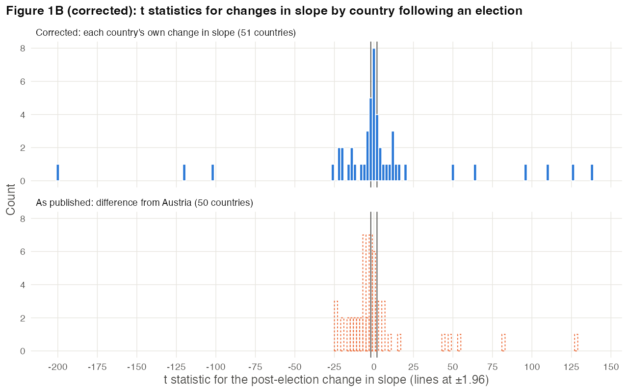
Basis Model, sample and clustered standard errors as in Figure_1.R; see the correction to the text on p. 4. The classification in Fig. 1A (21, 12 and 18 of 51 countries) reproduces and is unchanged.
p. 5, Fig. 2 caption
Published
Fig. 2. Effect of distance to/after election. Figure based on the loess models. For the figure based on ordinary least squares (OLS) ITS models, see fig. S1.
Correction
Fig. 2. Effect of distance to/after election. Panels A and B are based on loess models and panel C on a generalized additive model. For the figure based on ordinary least squares (OLS) ITS models, see fig. S2.
Basis Figure_2.R fits panel C (affective polarization) with method = 'gam'. Fig. S1 is the re-analysis of Michelitch and Utych (2018); the OLS ITS figure is fig. S2.
p. 6, Results
Published
Support for democratic norm violations increased very slightly but steadily from the pre-to the post-election, from a low of 0.40 in September to a high of 0.42 in March (βStd = 0.070, 95% CI [0.028, 0.113], P = 0.001).
Correction
Support for democratic norm violations increased slightly over the month before the election (pre-election slope βStd = 0.070, 95% CI [0.028, 0.113], P = 0.001). Between September and March, monthly means were lowest in October (0.40) and reached 0.42 in March.
Basis The coefficient is the pre-election slope from the model fitted to interviews within 33 days of the election, so its pre-election period runs from 6 October to Election Day; after the election the estimated slope is 0.016. Weighted monthly means of the 0-1 measure are 0.413 in September, 0.398 in October and 0.422 in March (unweighted: 0.403 in September, 0.388 in October).
p. 6, Results
Published
Furthermore, the results from the full, quadratic, and cubic models are all substantively similar to the linear model (see tables S3 to S5), which provides further confidence in the robustness of our findings.
Correction
The full, quadratic, and cubic models (see tables S3 to S5) do not all agree with the linear model. In the full-sample models (table S3), all three outcomes shift significantly at the election (support for political violence 0.065, support for norm violations 0.072, and affective polarization −3.59 thermometer points; each P < 0.001), and the slope for support for political violence changes significantly after the election (−0.203, P = 0.032). In the cubic model for support for norm violations (table S5), all three post-election slope terms are significant (P = 0.003 to 0.012).
Basis The table S3 shifts are small: 0.07, 0.08 and 0.11 standard deviations of the respective outcomes.
p. 9, Discussion
Published
We recognize that it is challenging to argue for a null result, but our design is especially well equipped to detect even minute exposure effects (Cohen’s d = 0.04). We obtained consistent null findings across three related measures of partisan animosity—affective polarization, support for norm violations, and support for political violence.
Correction
We recognize that it is challenging to argue for a null result. In our main models, the smallest effects detectable with 80% power at α = 0.05 are 0.086 to 0.094 standard deviations, and the power to detect an effect of Cohen’s d = 0.04 is 22% to 26%. Across three related measures of partisan animosity—affective polarization, support for norm violations, and support for political violence—we find at most small changes around the election.
Power of the main models (table S1, models 1, 3 and 5) for two-sided tests at α = 0.05. The change in slope is per unit of the scaled time variable. Outcome Term Standard error (SD) Power to detect d = 0.04 Effect detectable with 80% power (SD) Support for political violence Post-election jump 0.031 26% 0.086 Support for political violence Change in slope 0.031 25% 0.087 Support for norm violations Post-election jump 0.033 23% 0.093 Support for norm violations Change in slope 0.033 22% 0.094 Affective polarization Post-election jump 0.032 24% 0.090 Affective polarization Change in slope 0.033 23% 0.093 Basis Computed from the standard errors of the post-election jump and change in slope in table S1, models 1, 3 and 5 (0.031 to 0.033 standard deviations). The small changes are described in the correction to p. 1.
p. 10, Methods, The sample
Published
YouGov surveyed a total of 66,000 respondents between 16 September 2022 and 12 October 2023 [...] The mean age of respondents was 50.8 (SD = 17.8), with 53.8% female and 50.5% Democrats, 31.1% Republicans, and 18.4% Independents (pure independents were excluded from the sample and leaners were coded as partisans).
Correction
YouGov conducted a total of 66,000 interviews between 16 September 2022 and 12 October 2023 [...] The mean age of respondents was 50.8 (SD = 17.8), with 53.8% female and 60.0% Democrats and 40.0% Republicans (pure independents were excluded from the sample and leaners, 21.6% of respondents, were coded as partisans).
Basis The deposited norms file has 66,000 rows, one per interview, and the analysis file's 54,331 interviews come from 37,900 respondents. Counting leaners separately, the analysis file is 48.5% strong or weak Democrats, 29.9% strong or weak Republicans and 21.6% leaners; the published 50.5%, 31.1% and 18.4% match neither breakdown.
Supplementary information
SI section A.4, note to fig. S3
Published
Note: Figures based on the Interrupted time series (ITS) models presented in Table S5
Correction
Note: Figures based on the Interrupted time series (ITS) models presented in Table S6
Basis Table S5 holds the quadratic and cubic models; the models by number of races are in table S6.
SI section A.5, note to fig. S4
Published
Note: Figures based on the Interrupted time series (ITS) models presented in Table S7.
Correction
Note: Figures based on the Interrupted time series (ITS) models presented in Table S8.
Basis Table S7 holds the number-of-races models with corrected P values; the models by PVI are in table S8.
SI section B.1, Table S14
Published
Table S14 (“Sample Descriptives”), row “Age”: “Min” 18.00, “Mean” 50.82, “Max” 96.00, “SD” 17.76, “N” 54331.
Correction
Corrected Table S14. Age: Min 19.00, Mean 50.82, Max 97.00, SD 17.76, N 54331.
Corrected Table S14: every row describes the unadjusted values used in the models. Variable Min Mean Max SD N Age 19 50.82 97 17.76 54331 Gender 1 1.54 2 0.50 54331 PID 1 3.48 7 2.38 54331 Education 1 2.11 4 1.03 54331 Basis Table_S14.R subtracts 1 from age before describing it, which gives the published minimum and maximum and a mean of 49.82; the published mean is that of the unadjusted ages. The corrected row describes the unadjusted ages, which the models use and the Methods report (mean 50.8). The other rows are unchanged.
SI section B.5, Power Analysis
Published
Assuming an alpha of 0.05 and using 1000 simulations to run for each unique setting combination, Models 1, 3, and 5 (the models presented in the main text) have a statistical power of .94, .93, and .99, respectively (relative to the normal standard of .8). [...] The specific code can be found with our replication materials. [...] Nonetheless, for all three outcomes of interest, our models have a power of .99, assuming an alpha of 0.05. The specific code can be found with our replication materials.
Correction
Assuming an alpha of 0.05 and using 1000 simulations to run for each unique setting combination, Models 1, 3, and 5 (the models presented in the main text) have a statistical power of .94, .93, and .99, respectively (relative to the normal standard of .8); the effect size at which this power was evaluated is not reported. [...] The code for this analysis is not in the replication archive. [...] Nonetheless, for all three outcomes of interest, our models have a power of .99 to detect an effect of one-fourth of a standard deviation, assuming an alpha of 0.05. For an effect of Cohen’s d = 0.04, the power of Models 1, 3, and 5 is 22% to 26% (see the correction to the Discussion, p. 9). The code for this analysis is not in the replication archive.
Basis The Dataverse deposit (doi:10.7910/DVN/WAIING, version 1.0) contains no power-analysis code.