

The paper
Sean Jeremy Westwood, Solomon Messing, and Yphtach Lelkes (2020). Projecting Confidence: How the Probabilistic Horse Race Confuses and Demobilizes the Public. The Journal of Politics 82(4), 1530–1544.
doi:10.1086/708682 (opens in a new tab) · Replication data: doi:10.7910/DVN/TRIEF2 (opens in a new tab)
Main text
pp. 1534–1535, Study 1 design
Published
Our design relies on the fact that probabilistic forecasts present essentially the same information as vote share estimates with an accompanying margin of error in qualitatively different ways.
Correction
Our design relies on the fact that probabilistic forecasts and vote share estimates with an accompanying margin of error can be derived from the same polling data and presented in qualitatively different ways. In our stimuli the two formats did not carry the same information: the win probabilities reflect the spread of a single survey, while the margin of error reflects the precision of the average of 20 surveys (see the correction to p. 1535).
Basis The deposited simulation code (supp.r), also printed in SI section 3.1.1, computes the margin of error from the standard error of the mean of 20 simulated surveys and the win probabilities from that standard error multiplied by √20. The comparisons between display formats do not depend on this mapping. The accuracy benchmark on p. 1536 does.
p. 1535, Study 1 stimuli
Published
A plausible frequentist 95% confidence interval (CI) of ±2% was generated by simulating 20 surveys of 1,000 people (see the appendix, available online, for details). Based on the same variance estimates, we also estimated the probability that candidate A would get >50% of the vote and win the hypothetical election, which ranged from 13% to 87%.
Correction
A plausible frequentist 95% confidence interval (CI) of ±2% was generated by simulating 20 surveys of 1,000 people (see the appendix, available online, for details); its half-width, 2.09 percentage points, is 2.09 times the standard error of the 20-survey average (1.00 point). From the same simulated surveys, we also estimated the probability that candidate A would get >50% of the vote and win the hypothetical election, which ranged from 13% to 87%. These probabilities use the standard deviation of a single survey, 4.48 percentage points (√20 times the standard error), and so express the predictive uncertainty of one poll. The ±2% interval expresses the uncertainty of the 20-survey average. On the variance of the displayed interval, the probability that candidate A wins would be less than 0.001 at a 45% vote share and more than 0.999 at 55%.
Table A4 with an added column. Probability shown: 1 − Φ((0.5 − estimate)/σ) with σ = 0.0448, the standard deviation of a single simulated survey, as in the deposited code. Added column: σ = 0.0100, the standard error of the 20-survey average behind the ±2% interval. Estimate Margin of Error Probability shown Probability on the variance of the ±2% interval 0.45 0.02 0.13 < 0.001 0.46 0.02 0.19 < 0.001 0.47 0.02 0.25 0.001 0.48 0.02 0.33 0.023 0.49 0.02 0.41 0.159 0.51 0.02 0.59 0.841 0.52 0.02 0.67 0.977 0.53 0.02 0.75 0.999 0.54 0.02 0.81 > 0.999 0.55 0.02 0.87 > 0.999 Basis Computed from the deposited supp.r, which fixes the standard error at 1.00 point and sets sd = est_se * sqrt(N_survey) for the probabilities. The probabilities shown to participants reproduce Table A4 exactly.
p. 1535, note 9
Published
Results disaggregating these factors are consistent and are presented in tables A7 and A8.
Correction
Results disaggregating these factors are consistent and are presented in tables A8 and A9.
Basis Table A8 reports the display-order analysis and Table A9 the margin-of-error analysis.
p. 1535, Study 1 stimuli, probability of victory
Published
As is true of weighted, adjusted, and/or modeled estimate of
\hat{\mu}_vand\hat{\sigma}_v, the probability of victory, orP(\mu_v > .5)can then be estimated by1 - \Phi([\hat{\mu}_v - .5]/\hat{\sigma}_v).Correction
As is true of weighted, adjusted, and/or modeled estimate of
\hat{\mu}_vand\hat{\sigma}_v, the probability of victory, orP(\mu_v > .5)can then be estimated by1 - \Phi([.5 - \hat{\mu}_v]/\hat{\sigma}_v).Basis As printed, the expression equals
\Phi([.5 - \hat{\mu}_v]/\hat{\sigma}_v), the probability that candidate A receives less than half of the vote. With the standard deviation the deposited code uses (4.48 percentage points), it gives 0.13 at a 55% vote share, where Table A4 shows 0.87. The deposited supp.r computes the probabilities as1-pnorm(q = .5, mean = est, sd = est_se * sqrt(N_survey) ), which is1 - \Phi([.5 - \hat{\mu}_v]/\hat{\sigma}_v), the expression printed on p. 1532. The probabilities shown to participants do not change.p. 1536, Figure 3
Published
Figure 3, with the axis label “Proportion of respondents who vote conditioning on election year, prior turnout, and pid (95% Confidence Intervals)”.
Correction
Corrected Figure 3, estimated from Table A2 model 4, the model with election-year fixed effects that the axis label and the note to Figure A2 describe. Predicted turnout is 0.755 [0.749, 0.760] among respondents who expect a close race and 0.731 [0.721, 0.740] among those who expect the leading candidate to win by quite a bit, a difference of 2.4 percentage points.
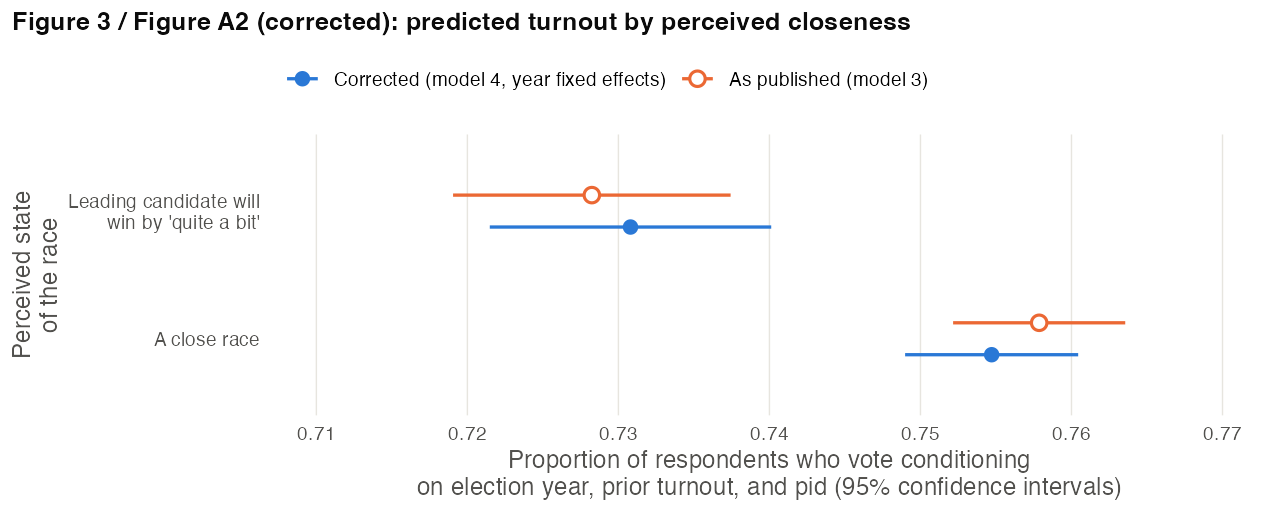
Basis The deposited supp.r draws the figure from model 3, which controls for the electoral college and popular vote margins in place of election year (0.758 and 0.728, a difference of 3.0 points). The model 4 difference agrees with the text's “about 2.5%” on p. 1533. Hollow points show the published estimates.
p. 1536, Study 1 results
Published
When presented with the commensurate 87% probability that candidate A would win, participants expected candidate A to get 64.6% of the vote (95% CI: 63.0%, 66.2%)—an 8 percentage point difference. [...] When presented with commensurate vote share estimates that put candidate A’s share of the vote at 55%, respondents were more than 27 percentage points off—the average participant reported a 59.6% likelihood that candidate A would win (95% CI: 58.1%, 61.0%).
Correction
When presented with the 87% probability that candidate A would win, which our design paired with a 55% vote share, participants expected candidate A to get 64.6% of the vote (95% CI: 63.0%, 66.2%)—an 8 percentage point difference. [...] When presented with vote share estimates that put candidate A’s share of the vote at 55%, the average participant reported a 59.6% likelihood that candidate A would win (95% CI: 58.1%, 61.0%), 27.4 percentage points below the paired 87% win probability and 40.4 points below the probability of more than 99.9% implied by a 55% share with a ±2% margin of error.
Basis The 87% probability and the ±2% margin of error were computed with different variances (see the correction to p. 1535), so the size of this error depends on which benchmark is used.
p. 1537, hypothetical vote intent
Published
After conditioning on past voting history and party, we observed preliminary evidence that participants were slightly less likely to say they would hypothetically vote when seeing more extreme probabilistic forecasts (table A9), though this finding should be considered exploratory.
Correction
After conditioning on a preelection rating of their own chance of voting in November 2016 and on party, we observed preliminary evidence that participants were slightly less likely to say they would hypothetically vote when seeing more extreme probabilistic forecasts (table A10), though this finding should be considered exploratory.
Basis The covariate is SCALE10_W21 from the archive's American Trends Panel wave 21 file (ATP W21.sav), labeled “Please rate your chance of voting in November on a scale of 10 to 1”. It records expected turnout in the 2016 election, asked before the election, and contains no information on past voting. The vote-intent models are in Table A10; Table A9 reports the margin-of-error analysis. The estimates do not change.
p. 1539, replication varying which candidate is reported ahead
Published
When the other candidate was reported to be ahead, respondents were less certain of victory (β = −0.19, T = −2.66, p < .009), reported a smaller expected vote share (β = −13.20, T = −2.50, p = .03), and a lower probability of victory (β = −15.22, T = −2.30, p = .02).
Correction
When the other candidate was reported to be ahead, respondents were less certain of victory (interaction of candidate B ahead and winning probability, β = −0.19, T = −2.66, p < .009), reported a smaller expected vote share (interaction β = −13.20, T = −2.25, p = .03), and a lower probability of victory (interaction β = −15.22, T = −2.30, p = .02).
Basis The three estimates are the Candidate B Ahead × Winning Probability interactions in Table A12; the Candidate B Ahead main effects (0.092, 1.604 and 7.025) are not statistically significant. Table A12 gives the vote-share interaction as −13.204 with standard error 5.871, so T = −2.25, which matches the reported p = .03 at 172 degrees of freedom. T = −2.50 would give p = .013. Table A12 reports 177 observations for certainty and probability of victory and 176 for vote share.
p. 1540, Study 2 results, robustness and note 15
Published
Comparing the standardized effects of probability and vote share likewise reveals that probability has a much larger effect (see table A18). [...] We found no significant main effect of numeracy and no interaction between numeracy and forecasted probabilities displayed in the game (see table A19). [...] Removing respondents who made such a mistake does not substantively impact our results (table A15). [...] We found no evidence of directional differences; see table A16.
Correction
Comparing the standardized effects of probability and vote share likewise reveals that probability has a much larger effect (see table A19). [...] We found no significant main effect of numeracy and no interaction between numeracy and forecasted probabilities displayed in the game (see table A20). [...] Removing respondents who made such a mistake does not substantively impact our results (table A16). [...] We found no evidence of directional differences; see table A18.
Basis In the SI, Table A16 removes respondents who mixed up probability and vote share, Table A18 tests for directionality, Table A19 reports normalized effects and Table A20 reports numeracy.
p. 1541, robustness (learning over rounds)
Published
Table A16 shows that there were no significant interactions between round and absolute distance between vote share and probabilistic forecast, suggesting that on average this did not affect our results.
Correction
Table A17 shows that there were no significant interactions between round and absolute distance between vote share and probabilistic forecast, suggesting that on average this did not affect our results.
Basis Table A17 (“Study 2 Model with Interactions”) reports the interactions of round with the absolute distances of the win probability and the vote share from 50%, and the SI text on p. 31 cites it for this result. Table A16 removes respondents who mixed up probability and vote share. The round-interaction model in the deposited supp.r reproduces Table A17.
p. 1541, group size study
Published
We do not find an effect of group N on behavior (table A20)
Correction
We do not find an effect of group N on behavior (table A21)
Basis Table A21 reports the group-size models.
p. 1542, order of probabilities and vote share
Published
We detected no effect of order on behavior (see table A20).
Correction
We detected no effect of order on behavior (see table A21).
Basis Column 2 of Table A21 reports the order interactions.
Supplementary information
SI p. 6, Figure A2
Published
Members of the public saying that they expect one candidate to ”Win by quite a bit” [...] are less likely to vote, even after conditioning on year, party, past voting (predicted proportions from model 4 in Table A2.
Correction
The plotted points come from model 3. Figure A2 is the same plot as Figure 3; the corrected version, from model 4 as this note states, is in the correction to p. 1536 (close race 0.755, win by quite a bit 0.731).
SI p. 7, Table A2, model 3
Published
Table A2, model (3): row ‘Win by quite a bit’ −0.030∗∗∗ (0.006); row “Electoral college margin” 0.092∗∗∗ (0.021); row “Popular vote margin” 0.0004 (0.093).
Correction
Corrected model 3. With the popular vote margin measured as the difference between the winner's and the runner-up's shares, the ‘win by quite a bit’ coefficient is −0.032*, the electoral college margin coefficient is −0.002 and the popular vote margin coefficient is 0.216*.
Table A2, model 3, with the popular vote margin measured as the absolute difference between the winner's and the runner-up's shares of the popular vote. Dependent variable: voted. Standard errors in parentheses; * p<0.05; ** p<0.01; * p<0.001. The first column reproduces the published model 3 from the deposited code. (3) as published (3) corrected ‘Win by quite a bit’ −0.030* (0.006) −0.032* (0.006) Prior turnout 0.448* (0.005) 0.448* (0.005) Independent −0.112* (0.009) −0.112* (0.009) Lean dem 0.003 (0.009) 0.003 (0.009) Lean rep 0.017 (0.009) 0.017 (0.009) Rep 0.024** (0.009) 0.025** (0.009) Strong dem 0.045* (0.008) 0.045* (0.008) Strong rep 0.069* (0.009) 0.069* (0.009) Electoral college margin 0.092* (0.021) −0.002 (0.043) Popular vote margin 0.0004 (0.093) 0.216* (0.092) Constant 0.407* (0.008) 0.410* (0.008) Observations 23,922 23,922 R2 0.258 0.258 Adjusted R2 0.257 0.257 Basis SI p. 6 describes the control as the absolute value of the popular vote margin. The deposited supp.r computes it as the absolute difference between the winner's share of the vote and 50%, which puts the 1996 margin at 0.8 points (actual margin 8.5) and the 2016 margin at 4.0 (actual 2.1). The actual margin is in the archive's electionwinners.csv (PV_Percent_Margin). Models 1, 2 and 4 do not use the margins and are unchanged.
SI p. 8, Figure A3
Published
Figure A3: Public expectations of large victories in presidential elections, 1952-2016
The series labeled “Popular vote margin”.
Correction
Corrected Figure A3, with the popular vote margin measured as the winner's share minus the runner-up's share. The margin is negative in 2000 and 2016, when the electoral college winner lost the popular vote. It was 3.9 points in 2012 and −2.1 in 2016.
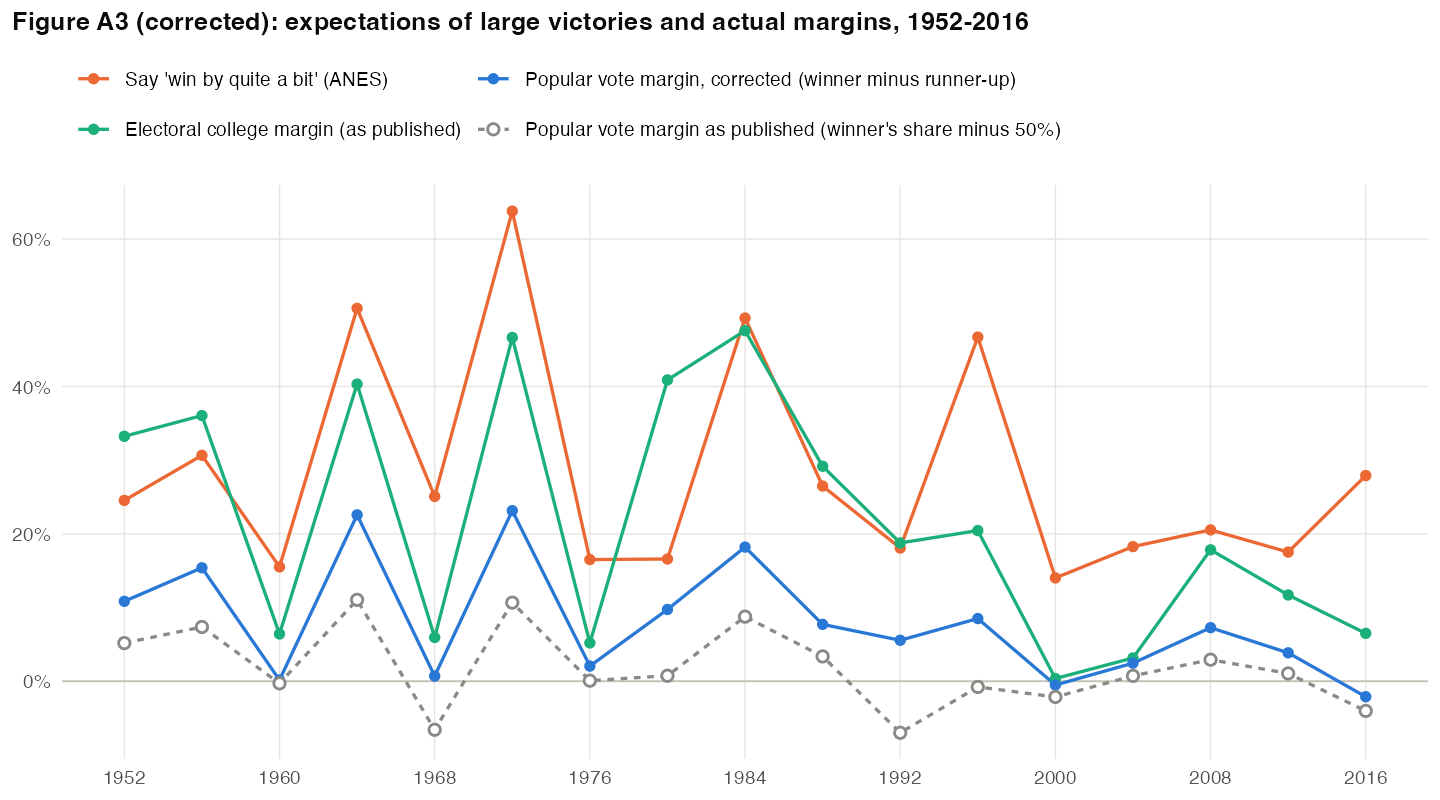
Basis The published series is the winner's share of the popular vote minus 50% (dashed grey line). See the correction to Table A2.
SI p. 11, section 3.1
Published
Based on that error, estimates of the probability that candidate A would win were then randomly assigned to values ranging from 13% to 87%.
Correction
Based on that error multiplied by √20, the standard deviation of a single simulated survey (4.48 percentage points), estimates of the probability that candidate A would win were then randomly assigned to values ranging from 13% to 87%. With the error behind the ±2% interval itself, the probabilities would range from less than 0.001 to more than 0.999 (see the correction to p. 1535).
Basis The code printed in section 3.1.1 computes the interval as qt(.975, df = N_survey) * est_se and the probabilities with sd = est_se * sqrt(N_survey).
SI pp. 11–12, section 3.1.1
Published
With this data in hand, the probability of victory, or
P(\mu_v > .5)can be estimated by1 - \Phi\left(\frac{\hat{\mu}_v - .5}{\hat{\sigma}_v}\right).Correction
With this data in hand, the probability of victory, or
P(\mu_v > .5)can be estimated by1 - \Phi\left(\frac{.5 - \hat{\mu}_v}{\hat{\sigma}_v}\right).Basis See the correction to p. 1535. The code printed below in the same section computes
est_prob <- 1-pnorm(q = .5, mean = est_vote_share, sd = est_se * sqrt(N_survey) ), which matches the corrected expression.SI p. 19, section 3.3
Published
With the addition of control variables—party and whether the respondent reported voting in 2016, we observe weak evidence (p = 0.11, two-tailed)
Correction
With the addition of control variables—party and the respondent's preelection rating of their chance of voting in November 2016 (1 to 10, American Trends Panel wave 21), we observe weak evidence (p = 0.11, two-tailed)
Basis See the correction to p. 1537.
SI p. 21, Table A10
Published
Table A10, row “Reported voting in 2016”.
Correction
Row label: “Preelection chance of voting in November 2016 (1–10, wave 21)”. The estimates are unchanged.
SI p. 22, section 3.4.1
Published
To simplify this study we only used two of the twenty numerical values for probability/vote share (45% and 55%).
Correction
To simplify this study we only used two of the 10 numerical values for probability/vote share (45% and 55%).
Basis Study 1 used 10 values (Table A4 and p. 1535).
SI p. 28, section 4.3
Published
Table A14 reports the model results used to generate Figure 3 in the main manuscript.
Correction
Table A14 reports the model results used to generate Figure 8 in the main manuscript.
Basis Figure 8 shows the Study 2 voting-game estimates; Figure 3 shows the ANES turnout estimates.
SI p. 31, Table A15
Published
Observations 1,171
Correction
Observations 5,845
Basis The model is estimated on 5,845 trials, as p. 1539 states; 1,171 is the number of respondents. The table's coefficients, R² and residual standard error reproduce from the archive's longform.RData on 5,845 trials.