

The paper
Samantha Goerger, Jonathan Mummolo, and Sean J. Westwood (2023). Which Police Departments Want Reform? Barriers to Evidence-Based Policymaking. Journal of Experimental Political Science 10(3), 403–412.
doi:10.1017/xps.2022.21 (opens in a new tab) · Replication data: doi:10.7910/DVN/IDAIUZ (opens in a new tab)
Main text
p. 404
Published
for example the discovery of sup-par performance, or even misconduct [...] could fail to generalize to organizations at large (Allcott 2017).
Correction
for example the discovery of sub-par performance, or even misconduct [...] could fail to generalize to organizations at large (Allcott 2015).
Basis Allcott’s “Site Selection Bias in Program Evaluation” appeared in The Quarterly Journal of Economics 130(3) in 2015.
p. 404
Published
An exception is the population size of jurisdictions – we find larger jurisdictions are less likely to respond affirmatively to our outreach efforts.
Correction
An exception is the population size of jurisdictions – we find smaller jurisdictions are less likely to respond affirmatively to our outreach efforts, although this association is not significant after correcting for multiple comparisons.
Basis The median split in figure2.R writes “Low” and “High” into each numeric covariate one value at a time, so after the first assignment the vector is text and the remaining values are compared with the median as strings. In the public ag.csv this codes 2,896 agencies as above the median population and 46 as below; 51% land on the correct side. lm() then takes “High” as the reference level, so the published −14.84 is a below-minus-above difference on this misclassified split. With a correct above-median indicator, and the published weights and standard errors, the estimate is +7.14 percentage points (SE 3.20; see the correction to p. 407).
p. 407
Published
Across the 44 test results in this figure, only one covariate, population of the jurisdiction, was significantly associated with responses in either the control or treatment groups. Specifically, moving from below to above the median jurisdiction population in our sample is associated with a 14.84 percentage point decrease in the probability of an affirmative response (BH-corrected p-value = 0.01).
Correction
Across the 44 test results in this figure, no covariate was significantly associated with responses in the control group. Moving from below to above the median jurisdiction population in our sample is associated with a 7.14 percentage point increase in the probability of an affirmative response (uncorrected p-value = 0.03; BH-corrected p-value = 0.32). In the treatment group (Appendix Figure E1), two covariates were significantly associated with responses: officers killed by felons per capita (−13.12 percentage points, BH-corrected p-value = 0.01) and officers killed in accidents per capita (−13.25 percentage points, BH-corrected p-value = 0.01).
Basis Estimates use a correct above-median indicator (see the correction to p. 404), with the published population weights, HC3 standard errors and Benjamini-Hochberg correction across all 88 coefficients. The published SI Table E2 already listed the two treatment-group covariates as significant (13.12 and 13.25, BH-corrected p = 0.01); with the corrected split their estimates keep the same size and change sign.
pp. 407–408
Published
While larger jurisdictions are less likely to show interest in research collaborations – an important limitation that could stymie partnerships in major departments – the overall pattern of results does not indicate selection related to agency performance
Correction
While smaller jurisdictions are less likely to show interest in research collaborations, and few of the very largest departments agreed, the overall pattern of results does not indicate selection related to agency performance
Basis In the control group, 2.9% of agencies in the smallest tenth of jurisdictions by population agreed, against 8.8% below the median and 20.8% above it. Among control-group agencies serving more than 500,000 people, 2 of 16 agreed; among those serving more than one million, 0 of 5.
p. 408, Figure 2
Published
Figure 2. Agency and jurisdiction attributes do not predict affirmative responses.
Figure 2, horizontal axis: “Percentage−point change in agreement from a one standard deviation increase in the predictor”
Correction
Corrected Figure 2, estimated with a correct above-median indicator. The horizontal axis is the percentage-point difference in agreement between agencies above and below the median of each predictor. No predictor has a Benjamini-Hochberg corrected p-value below .05.
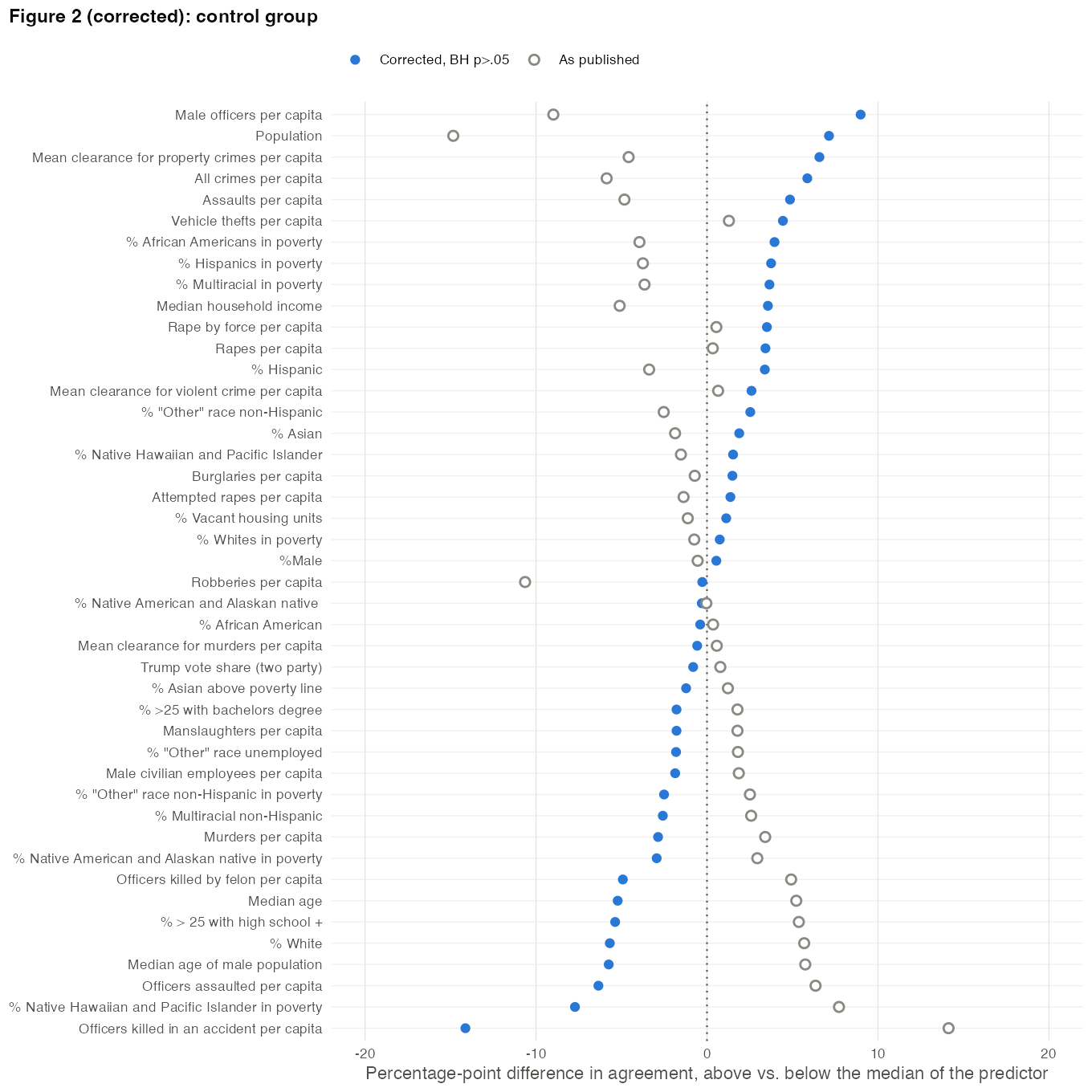
Basis Hollow points show the published estimates. Footnote 5 and the text on p. 407 describe the predictors as above-median indicators; the published axis label describes standardized predictors, which figure2.R does not use.
p. 409
Published
agencies told their rank on violent crime clearance rates were about 8 percentage points (SE = 0.01) less likely to say they would discuss a potential collaboration.
Correction
agencies told their rank on violent crime clearance rates were about 8 percentage points (SE = 0.02, clustered by matched pair) less likely to say they would discuss a potential collaboration.
Basis SI Table E4, column 2, and Figure 3 report this estimate (−7.98 percentage points) with a standard error of 0.0174, clustered by matched pair with rddtools::vcovCluster, which counts the 1,241 pair indicators in its small-sample correction. A cluster-robust standard error that does not count indicators nested within clusters is 0.0123. The estimate is significant under either.
p. 410, Discussion and conclusion
Published
An exception pertains to the population size of jurisdictions, with larger jurisdictions responding affirmatively less often than smaller ones.
Correction
An exception pertains to the population size of jurisdictions, with smaller jurisdictions responding affirmatively less often than larger ones, although this association is not significant after correcting for multiple comparisons. The very largest agencies are an exception: 2 of the 16 control-group agencies serving more than 500,000 people agreed, against 20.8% of agencies above the median population.
Basis See the corrections to pp. 404 and 407.
p. 411, data availability statement and references
Published
Goerger, Mummolo, and Westwod (2022). Allcott, Hunt. 2017. Site Selection Bias in Program Evaluation. The Quarterly Journal of Economics 130(3): 1117–65.
Correction
Goerger, Mummolo, and Westwood (2022).
Allcott, Hunt. 2015. Site Selection Bias in Program Evaluation. The Quarterly Journal of Economics 130(3): 1117–65.
p. 412, references
Published
Gelman, Andrew, Jeffrey Fagan and Alex Kiss. 2007. [...] Journal of the American Statistical Association 102(429): 813–23. Goerger, Samantha, Jonathan Mummolo and Sean J. Westwod. 2022. Replication Data for: [...]
Correction
Gelman, Andrew, Jeffrey Fagan and Alex Kiss. 2007. [...] Journal of the American Statistical Association 102(479): 813–23.
Goerger, Samantha, Jonathan Mummolo and Sean J. Westwood. 2022. Replication Data for: [...]
Supplementary information
SI pp. 20–25, Table E2
Published
Table E2: Estimates from Figure 2: Correlates of responding
Table E2 has 88 rows; the first rows are “Population” −14.84 (Control), “Officers killed by felon per capita” 13.12 (Treatment) and “Officers killed in an accident per capita” 13.25 (Treatment).
Correction
Corrected Table E2. No control-group covariate has a Benjamini-Hochberg corrected p-value below .05; in the treatment group, officers killed by felons per capita (−13.12) and officers killed in accidents per capita (−13.25) do. The treatment-group population estimate is 7.01 (published: 57.70).
Corrected Table E2: bivariate regressions of agreement on an indicator for being above the median of each covariate, weighted by jurisdiction population, HC3 standard errors; Benjamini-Hochberg correction across all 88 coefficients. Estimates in percentage points. Variable Estimate Uncorrected p-value Benjamini-Hochberg corrected p-value Condition Officers killed by felon per capita −13.12 0.00 0.01 Treatment Officers killed in an accident per capita −13.25 0.00 0.01 Treatment %Male 0.55 0.92 0.96 Control % White −5.68 0.19 0.80 Control % African American −0.40 0.93 0.96 Control % Native American and Alaskan native −0.30 0.96 0.96 Control % Asian 1.89 0.65 0.94 Control % Native Hawaiian and Pacific Islander 1.53 0.69 0.94 Control % "Other" race non-Hispanic 2.53 0.49 0.94 Control % Multiracial non-Hispanic −2.58 0.63 0.94 Control % Hispanic 3.38 0.46 0.94 Control % > 25 with high school + −5.37 0.21 0.80 Control % >25 with bachelors degree −1.78 0.72 0.94 Control % "Other" race unemployed −1.81 0.64 0.94 Control % Whites in poverty 0.75 0.89 0.96 Control % African Americans in poverty 3.95 0.41 0.94 Control % Native American and Alaskan native in poverty −2.94 0.55 0.94 Control % Asian above poverty line −1.22 0.77 0.94 Control % Native Hawaiian and Pacific Islander in poverty −7.72 0.24 0.80 Control % "Other" race non-Hispanic in poverty −2.51 0.57 0.94 Control % Multiracial in poverty 3.65 0.45 0.94 Control % Hispanics in poverty 3.75 0.45 0.94 Control % Vacant housing units 1.12 0.83 0.96 Control Male officers per capita 8.99 0.20 0.80 Control Male civilian employees per capita −1.86 0.68 0.94 Control Officers killed by felon per capita −4.92 0.67 0.94 Control Officers assaulted per capita −6.35 0.23 0.80 Control Murders per capita −2.86 0.70 0.94 Control Manslaughters per capita −1.78 0.77 0.94 Control Rapes per capita 3.42 0.52 0.94 Control Rape by force per capita 3.50 0.51 0.94 Control Attempted rapes per capita 1.37 0.75 0.94 Control Robberies per capita −0.28 0.96 0.96 Control Assaults per capita 4.86 0.37 0.94 Control Burglaries per capita 1.49 0.78 0.94 Control Vehicle thefts per capita 4.44 0.41 0.94 Control All crimes per capita 5.87 0.28 0.84 Control Mean clearance for murders per capita −0.57 0.89 0.96 Control Mean clearance for violent crime per capita 2.60 0.63 0.94 Control Mean clearance for property crimes per capita 6.58 0.23 0.80 Control Median age −5.22 0.26 0.82 Control Median age of male population −5.75 0.21 0.80 Control Median household income 3.56 0.51 0.94 Control Trump vote share (two party) −0.81 0.86 0.96 Control Population 7.14 0.03 0.32 Control Officers killed in an accident per capita −14.13 0.01 0.21 Control Population 7.01 0.05 0.44 Treatment %Male −1.43 0.84 0.96 Treatment % White −8.57 0.08 0.50 Treatment % African American 1.16 0.86 0.96 Treatment % Native American and Alaskan native 2.20 0.76 0.94 Treatment % Asian 5.93 0.25 0.80 Treatment % Native Hawaiian and Pacific Islander 7.89 0.07 0.49 Treatment % "Other" race non-Hispanic 7.25 0.08 0.50 Treatment % Multiracial non-Hispanic 5.64 0.34 0.94 Treatment % > 25 with high school + −3.66 0.55 0.94 Treatment % >25 with bachelors degree 3.13 0.60 0.94 Treatment % Whites in poverty −3.16 0.64 0.94 Treatment % African Americans in poverty 2.42 0.73 0.94 Treatment % Asian above poverty line 6.45 0.19 0.80 Treatment % Native Hawaiian and Pacific Islander in poverty 3.58 0.57 0.94 Treatment % Multiracial in poverty 1.75 0.81 0.96 Treatment % Hispanics in poverty 3.92 0.55 0.94 Treatment % Vacant housing units −1.29 0.84 0.96 Treatment Male officers per capita −6.42 0.19 0.80 Treatment Male civilian employees per capita 6.69 0.16 0.80 Treatment Officers assaulted per capita 9.86 0.11 0.66 Treatment Murders per capita −0.49 0.95 0.96 Treatment Manslaughters per capita 3.80 0.59 0.94 Treatment Rapes per capita 3.45 0.59 0.94 Treatment Rape by force per capita 3.02 0.64 0.94 Treatment Attempted rapes per capita 7.02 0.14 0.79 Treatment Robberies per capita −4.27 0.52 0.94 Treatment Assaults per capita −5.68 0.36 0.94 Treatment Burglaries per capita −6.31 0.30 0.86 Treatment Vehicle thefts per capita −6.54 0.30 0.86 Treatment All crimes per capita −4.41 0.46 0.94 Treatment Mean clearance for violent crime per capita 0.91 0.89 0.96 Treatment Mean clearance for property crimes per capita −4.59 0.45 0.94 Treatment Median age −2.15 0.73 0.94 Treatment Median age of male population −2.42 0.69 0.94 Treatment Median household income 0.49 0.94 0.96 Treatment % Hispanic 10.96 0.02 0.32 Treatment % "Other" race unemployed 9.16 0.03 0.32 Treatment % Native American and Alaskan native in poverty 10.11 0.05 0.41 Treatment % "Other" race non-Hispanic in poverty 10.65 0.02 0.32 Treatment Mean clearance for murders per capita 12.29 0.00 0.07 Treatment Trump vote share (two party) −10.42 0.04 0.38 Treatment Basis See the correction to p. 404. Rows follow the ordering rule of figure2.R.
SI p. 26, Figure E1
Published
Figure E1: Alternative Figure 2 Showing Effects Among the Treated
Figure E1, horizontal axis: “Percentage−point change in agreement from a one standard deviation increase in the predictor”
Correction
Corrected Figure E1, estimated with a correct above-median indicator and labelled as an above-versus-below-median difference.
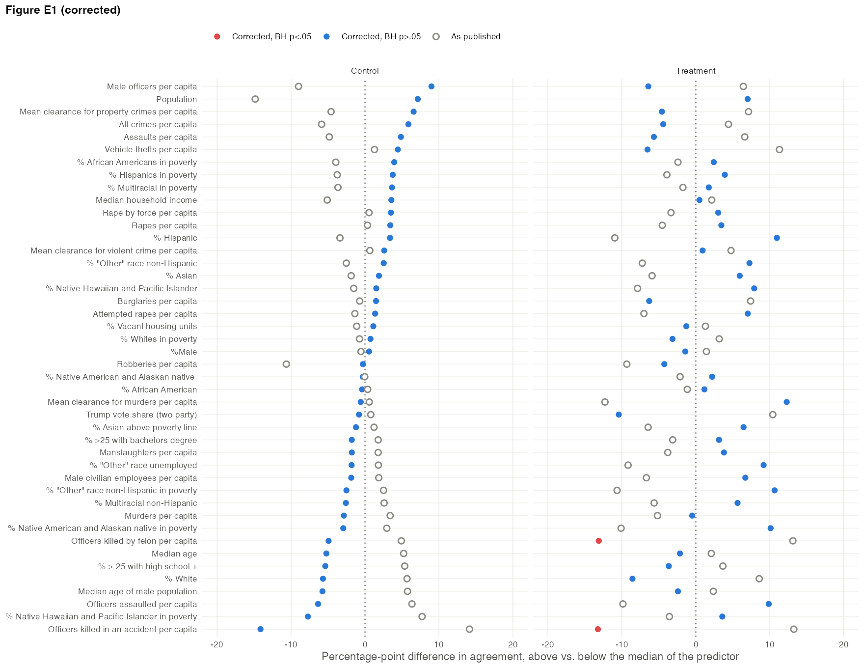
Basis Hollow points show the published estimates. The published treatment-group population estimate (57.70) lies outside the plotted range.
SI p. 27, Table E3, column 3
Published
Table E3, column 3: “Middle Rank Tercile” −0.05 (0.04); “Top Rank Tercile” 0.07 (0.05); “Confidential Condition X Middle Rank Tercile” 0.07 (0.04); “Ranking Condition X Middle Rank Tercile” −0.01 (0.05)
Correction
Corrected Table E3. Column 3 enters the rank tercile as a single linear term, so its four rows are the tercile slope and its interactions with the three conditions.
Corrected Table E3: row labels matched to the estimated terms. Column 3 enters the use-of-force rank tercile as a single linear term (1 = the third of agencies with the highest rates of using force, 3 = the lowest). Numeric Rank: 1 = highest rate of using force. HC1 standard errors in parentheses; * p<0.05; ** p<0.01; * p<0.001. Term (1) (2) (3) Intercept 0.13* (0.03) 0.21** (0.07) 0.23** (0.09) Confidential Condition −0.02 (0.04) −0.14 (0.09) −0.16 (0.12) Ranking Condition −0.09* (0.04) −0.17* (0.08) −0.22* (0.10) Ranking and Anonymous Condition −0.04 (0.04) −0.04 (0.10) −0.02 (0.12) Numeric Rank −0.0003 (0.0003) Confidential Condition X Numeric Rank 0.001 (0.0003) Ranking Condition X Numeric Rank 0.0004 (0.0003) Ranking and Anonymous Condition X Numeric Rank 0.0000 (0.0003) Rank Tercile (1, 2, 3) −0.05 (0.04) Confidential Condition X Rank Tercile 0.07 (0.05) Ranking Condition X Rank Tercile 0.07 (0.04) Ranking and Anonymous Condition X Rank Tercile −0.01 (0.05) Observations 462 462 462 R2 0.01 0.02 0.02 Basis In new_jersey_data.csv, t_rank is stored as the number 1, 2 or 3, so condition*t_rank fits one tercile term and one interaction per condition. The row labels in tablee3.R assume separate middle and top tercile indicators, which shifts every label in column 3. The estimates are unchanged.
SI p. 28, Table E4, columns 3 and 4
Published
Table E4, column 3: “Numeric Rank” 0.0000 (0.0000) and “Top Rank Tercile” −0.0000 (0.0000); column 4: “Middle Rank Tercile” 0.02 (0.02) and “Ranking Condition X Numeric Rank” −0.01 (0.03)
Correction
Corrected Table E4. In column 3, the row printed as “Top Rank Tercile” is the Ranking Condition × numeric rank interaction. In column 4, “Middle Rank Tercile” is the linear rank-tercile term and “Ranking Condition X Numeric Rank” is the Ranking Condition × tercile interaction.
Corrected Table E4: row labels matched to the estimated terms. Column 3 interacts the Ranking Condition with the numeric clearance rank and column 4 with the rank tercile entered as a single linear term (rank 1 and tercile 1 = the highest share of violent crimes cleared). Standard errors in parentheses: HC1 in column 1, clustered by matched pair in columns 2-4 (rddtools::vcovCluster, as in the published table); * p<0.05; ** p<0.01; * p<0.001. Term (1) (2) (3) (4) Intercept 0.15* (0.01) 0.04* (0.01) 0.01 (0.04) −0.01 (0.05) Ranking Condition −0.08* (0.01) −0.08* (0.02) −0.07 (0.04) −0.05 (0.06) Numeric Rank 0.0000 (0.0000) Rank Tercile (1, 2, 3) 0.02 (0.02) Ranking Condition X Numeric Rank −0.0000 (0.0000) Ranking Condition X Rank Tercile −0.01 (0.03) Matched Pair FE No Yes Yes Yes Observations 2,482 2,482 2,482 2,482 R2 0.02 0.52 0.52 0.52 Basis In national_data.csv, ranktercile is stored as the number 1, 2 or 3, so condition*ranktercile fits one tercile term and one interaction. The estimates are unchanged.
SI p. 43, Table J1, columns 3 and 4
Published
Table J1, column 3: “Top Rank Tercile” −0.0000 (0.0000); column 4: “Middle Rank Tercile” 0.02 (0.02) and “Ranking Condition X Numeric Rank” −0.02 (0.03)
Correction
Corrected Table J1, labelled as in the corrected Table E4.
Corrected Table J1 (agency coded as agreeing): row labels matched to the estimated terms. Column 3 interacts the Ranking Condition with the numeric clearance rank and column 4 with the rank tercile entered as a single linear term (rank 1 and tercile 1 = the highest share of violent crimes cleared). Standard errors in parentheses: HC1 in column 1, clustered by matched pair in columns 2-4 (rddtools::vcovCluster, as in the published table); * p<0.05; ** p<0.01; * p<0.001. Term (1) (2) (3) (4) Intercept 0.15* (0.01) 0.04* (0.01) 0.01 (0.04) −0.01 (0.05) Ranking Condition −0.08* (0.01) −0.08* (0.02) −0.06 (0.04) −0.05 (0.06) Numeric Rank 0.0000 (0.0000) Rank Tercile (1, 2, 3) 0.02 (0.02) Ranking Condition X Numeric Rank −0.0000 (0.0000) Ranking Condition X Rank Tercile −0.02 (0.03) Matched Pair FE No Yes Yes Yes Observations 2,482 2,482 2,482 2,482 R2 0.02 0.52 0.52 0.52 Basis tablej1.R uses the same models and row labels as tablee4.R. The estimates are unchanged.
SI p. 44, Table K1
Published
Table K1, columns 1 and 2: “Intercept” 0.24∗∗∗ and 0.12; “Numeric Rank” −0.02 (0.05) and −0.02 (0.08); “Sheriff Department” 0.02 (0.03) and 0.04 (0.05)
Correction
Corrected Table K1. The row printed as “Numeric Rank” is the agency-type term and the row printed as “Sheriff Department” is the Ranking Condition × agency-type interaction. The reference category is sheriff departments, so the agency-type term compares local police departments with sheriff departments (0.002 in the control group), and the interaction is the difference in the ranking effect between police and sheriff departments (0.019, p = 0.50).
Corrected Table K1: reference category sheriff departments (SAMPTYPE = 1, recorded as sheriff's offices in ag.csv); Police Department = local police departments (SAMPTYPE = 3); condition entered as a treatment indicator. Standard errors in parentheses: HC1 in column 1, clustered by matched pair in column 2; * p<0.05; ** p<0.01; * p<0.001. Term (1) (2) Intercept 0.15* (0.02) 0.01 (0.04) Ranking Condition −0.09* (0.02) −0.11** (0.04) Police Department 0.002 (0.02) 0.03 (0.04) Ranking Condition X Police Department 0.02 (0.03) 0.04 (0.05) Matched Pair FE No Yes Observations 2,462 2,462 R2 0.02 0.54 Basis The models contain no rank variable. In national_data_sheriff.csv, SAMPTYPE is 1 for the 602 agencies that ag.csv records as sheriff’s offices and 3 for the 1,860 local police departments. tablek1.R also enters condition as the number 1 or 2, so its intercept and agency-type rows describe a condition coded 0; the corrected table enters condition as a treatment indicator. The Ranking Condition and interaction estimates are unchanged.
Replication archive
Replication archive, figure2.R (treatment-group loop)
Published
lb[i+44]<-coef[i]-1.96se[i] ub[i+44]<-coef[i]+1.96se[i] sig[i+44]<-I(lb[i]*ub[i]>0)
Correction
lb[i+44]<-coef[i+44]-1.96se[i+44] ub[i+44]<-coef[i+44]+1.96se[i+44] sig[i+44]<-I(lb[i+44]*ub[i+44]>0)
Basis The treatment-group intervals and flag were computed from the control-group estimates. They set only the order in which results are sorted; the plotted estimates and the Benjamini-Hochberg colours do not use them. The Benjamini-Hochberg correction in figure2.R runs over all 88 coefficients, 44 covariates in each of the control and treatment groups.